Fault Prediction from Seismic Data - Deep Neural Network
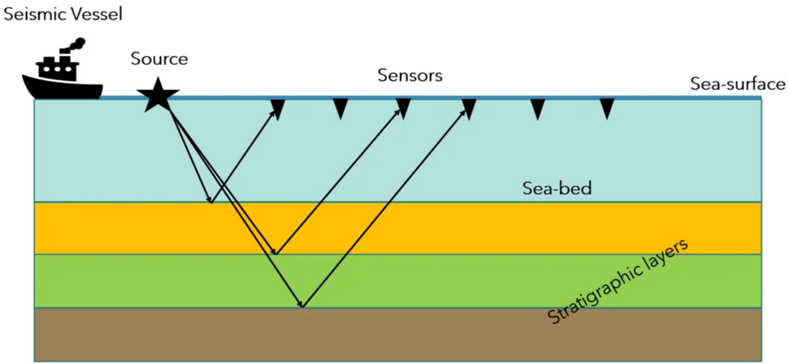
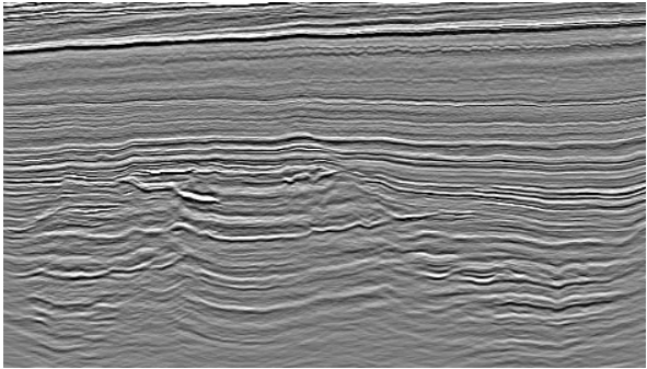
Seismic image gives a structural snapshot of the Earth’s subsurface at a time. A sound wave is sent to the subsurface from a ‘source’, which travels through the Earth’s layer at different velocity and gets reflected, refracted or diffracted along its way. In seismic imaging, we record the waves that are reflected back from different geological layers and stack them to create a 2D or 3D image. Because different geological layers have different physical properties, at the boundary between layers, the waves are reflected due to density contrast. There are different kinds of waves, but in imaging we are mostly focused on P-waves (compressional waves). The cartoon below gives you an example of seismic acquisition and actual image after collecting all the waves.
So whose fault is it?
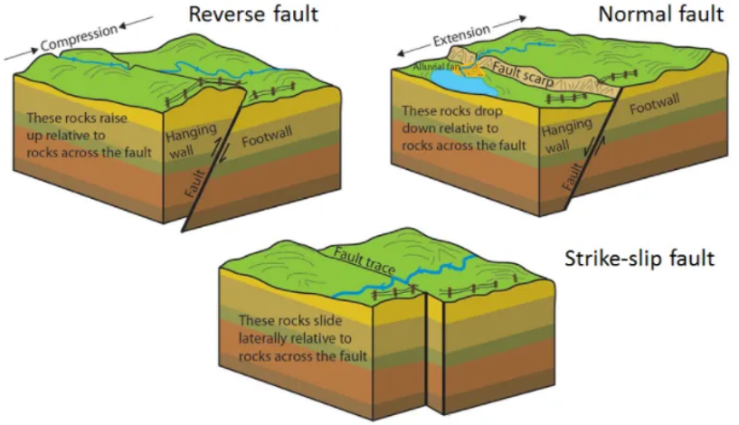
Faults are geological structures created by a combination of numerous physical processes such as pressures, gravity, plate tectonics etc. These are the cracks or planes along which block of rocks slips across. Faults comes in all kind of sizes, from few meters to miles. The San Andreas Fault is an example of very large scale strike-slip faulting (also called Transform Fault).
There are three major types of faults as shown in below:
Significance of Fault Mapping in seismic data
Fault mapping is one of the important aspects of seismic exploration as the careful analysis of faults may help in understanding if there is likelihood of finding oil/gas reservoir in the subsurface. In the early exploration phase, two points are critical:
- ffaults may act as conduits for hydrocarbon to migrate
- they may help to trap oil in-place
During the oil/gas development phase, mapping of faults is critical in making economic analysis because faults influence the hydrodynamics of a reservoir by altering the fluid permeability. This will directly influence the volumetric of an oil/gas play as well mechanical engineering aspect of the oilfield development. In shallow subsurface, presence of faults pose danger to drilling. A correct identification of faults will allow to steer drilling bits such that any faulted region is avoided as much as possible.
Finally, large scale fault mapping helps to understand regional geodynamic process happening in the earth. This is critical in understanding natural hazards such as earthquakes, volcanoes, landslides etc.
We can see there are many benefits of fault identification, especially in the hydrocarbon exploration. Therefore a lot of effort has been made in the seismic exploration to accurately identify and map the faults. However, manual mapping of the faults is a tedious process and takes many days or weeks even in a small survey area.
So, can we use an aid from Machine Learning to expedite fault identification?
Fault Mapping and Prediction
With the advancement in Deep Neural Network, it might be possible to train seismic images to create a model that may be able identify Faults in the seismic data. In this article, I would like to walk you through a Deep Learning Framework that can predict the Faults from the seismic data. For this study, I used a synthetic seismic data provided by Force Competition (www.xeek.ai).
Data Exploration
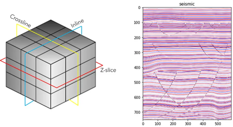
The data for this study comes in a SEG-Y format which is industry standard for seismic data (SEG stands for Society of Exploration Geophysicists). This is specialized data format and I used a python library called ‘segyio’ designed to read this type of data. Since I am using a 3D dataset, the segyio can readily convert the data into a 3D NumPy array. An example of 3D grid structure is shown below which also shows three planar surfaces: inline, crossline & z-slice. These are the 2D surfaces commonly used in seismic industries to visualize the data. A link to my github page will be provided at the end of this article for the full notebook.
Deep Convolution Network
The fault mapping can be categorized as a type of image segmentation task. Since, we want the output of the neural network to be full resolution image, a U-Net framework is suitable for this type of task. The U-Net framework was originally developed for image segmentation task in the field of Biomedical technology. A general schematics of the U-Net framework is shown below:
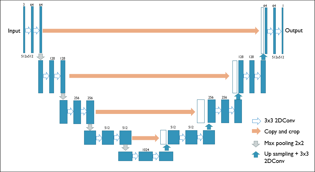
The U-Net has two distinct flow paths:
i) a forward path of contraction involving several downsampling steps. This is the encoder section of the U-Net which involves two 3x3 convolutions followed by a ReLU, a 2x2 max pooling and a stride of 2 for downsampling. The original U-Net implementation uses an ‘unpadded’ convolutions which result into reduced size of the final output.
ii) a reverse path of expansion involving several upsampling steps. This is the decoder section consisting of an upsampling of feature map, a 3x3 convolution and a concatenation of a feature map from the previous contracting block followed by 3x3 convolutions each with ReLU activation.
The code snippets for these two steps are below:
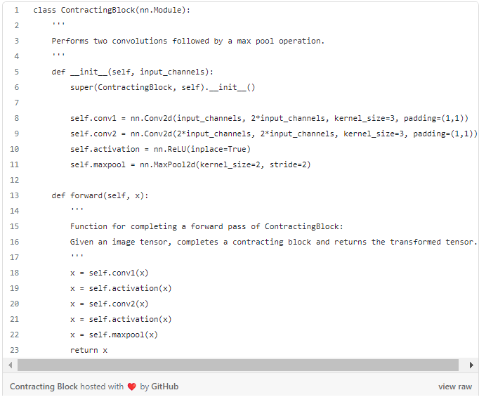
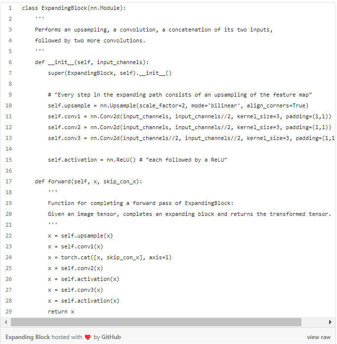
Where,
x: image tensor of shape (batch size, channels, height, width) skip_con_x: the image tensor from the contracting path
Note: In the original U-Net implementation, the output shape is smaller than the input, which requires a skip connection layer size to be matched with current layer. In this case, the skip-connection layer should be cropped to match the size of the layer after upsampling and convolution. Furthermore, the padding needs to be set to 1 to make sure the final output shape matches with input shape.
Next, we need a final code block that will output tensors with same input size.
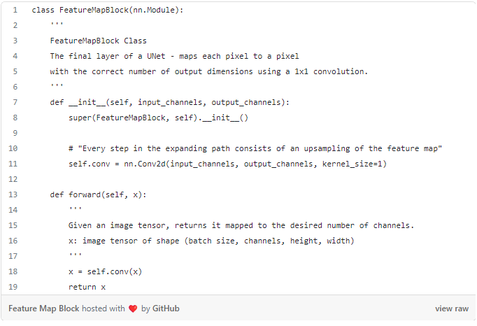
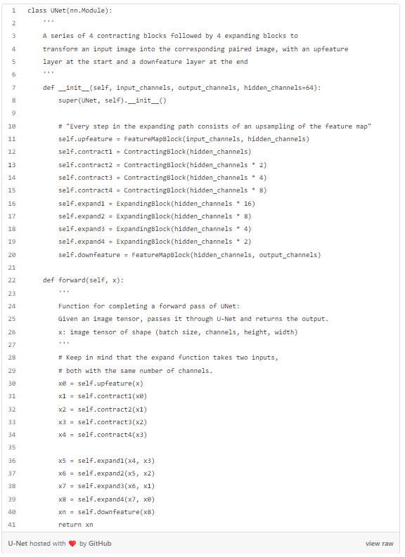
Putting altogether, the final U-Net block has 4 contraction and 4 expansion block and feature map block at the beginning and start of the network.
Training Data
I will be using two volumes of data for this study: a seismic cube and fault cube, where the seismic cube will be a training data and fault cube will be a label data. The fault data has a series of manually mapped surfaces which has been 0 and 1. The image on the left is a 2D seismic display in the inline direction where as on the right is the same display overlain with faults.
Can you notice the actual appearance of faults on the left image?
The original input data provided has the shape of (101, 589, 751). This means there are 101 inlines, 589 crosslines and 751 samples. Note that the seismic images are not RGB images, therefore they can be treated as a single channel grayscale images. The number of inlines can be treated as batch size, and along the inline we will have 2D image of shape 589 x 751 pixels.
The desired input tensor size is : (batch size, channels, height, width).
So, our input tensors is of shape (101, 1, 589, 751), where 1 is for single channel. However, the odd number size initially caused some problems, which led me to crop the input volume to get a shape of (101, 1, 512, 512)Model Training
The general training parameters are listed below. As of now, I have only trained the model with maximum epochs of 25, but we will see that for this dataset, the model starts to pick the faults very effectively at around 10 epochs. I ran the model on NVIDIA GeForce RTX 2060 Super with 8GB memory with batch size of 1 at a time.

Result
The images below are collected randomly at 3 different epochs. Notice, at Epoch of 4, the model is already starting to get a sense of faults and by Epoch of 19, it has managed to map the fault very closely.
If we look at the model performance, the loss function drops dramatically within the 5 Epochs and remains stable about 15 Epochs. Such quick drop in model loss is probably because of the clean synthetic data used for training.
Summary
This little experiment has demonstrated the power of deep learning and how it can be used to map the Faults relatively quickly given that the input data is noise free. However, in the real world, the seismic data are very messy and full of noises that may cause a significant roadblock to model accuracy. If we train the model using wide varieties of seismic datasets from the different basins all around the world, the model can generalize pretty well. In the next part, I will be focusing on implementing this model on a real world dataset provide by Schlumberger for this competition.